Understanding Gaussian Blurs

Let’s take a detailed look at the implementation behind Gaussian blurs. It’s the image processing algorithm that enables image manipulations like this:

We’ll start by reviewing Gaussian distributions and image convolution – the driving forces behind Gaussian blurs. Then, we’ll implement our own Gaussian blur algorithm from scratch with Swift. 

If you haven’t already read my article about edge detection in images, I’d recommend you read that first. It’ll help establish a foundation around convolution and the fundamentals of image processing. 

Convolution

In simple terms, convolution is simply the process of taking a small matrix called the kernel and running it over all the pixels in an image. At every pixel, we’ll perform some math operation involving the values in the convolution matrix and the values of a pixel and its surroundings to determine the value for a pixel in the output image.

By changing the values in the kernel, we can change the effect on the image – blurring, sharpening, edge detection, noise reduction, etc.

Convolution will be clearer once we see an example.

Gaussian Distributions

Next, let’s turn to the Gaussian part of the Gaussian blur. Gaussian blur is simply a method of blurring an image through the use of a Gaussian function.

You may have heard the term Gaussian before in reference to a Gaussian distribution (a.k.a. normal distribution).

Below, you’ll see a 2D Gaussian distribution. Notice that there is a peak in the center and the curve flattens out as you move towards the edges. 

Imagine that this distribution is superimposed over a group of pixels in an image. It should be apparent looking at this graph, that if we took a weighted average of the pixel’s values and the height of the curve at that point, the pixels in the center of the group would contribute most significantly to the resulting value. This is, in essence, how Gaussian blur works.

TLDR: A Gaussian blur is applied by convolving the image with a Gaussian function.

In English, this means that we’ll take the Gaussian function and we’ll generate an n x m matrix. Using this matrix and the height of the Gaussian distribution at that pixel location, we’ll compute new RGB values for the blurred image.

Overview

To start off, we’ll need the Gaussian function in two dimensions: 

The values from this function will create the convolution matrix / kernel that we’ll apply to every pixel in the original image. The kernel is typically quite small – the larger it is the more computation we have to do at every pixel. 

x and y specify the delta from the center pixel (0, 0). For example, if the selected radius for the kernel was 3, x and y would range from -3 to 3 (inclusive). 

σ – the standard deviation – influences how significantly the center pixel’s neighboring pixels affect the computations result. 

Technically, in a Gaussian function, because it extends infinitely, you could argue that you’d need to consider every pixel in the image to get the “correct” blur effect, but in practice pixels beyond 3σ have very little impact on the resulting values.

Implementation

We’re almost ready to start the implementation.

We’ll need to create a separate output image. We can’t modify the source image directly because changing the pixel values will mess up the math for the adjacent pixel’s computation in the next iteration.

Finally, we need to consider how we’ll handle the edges. If we were looking at the very first pixel in an image, the kernel would extend beyond the bounds of the image. As a result, implementations will commonly ignore the outer most set of pixels, duplicate the edge, or wrap the image around.

In our case, for ease of implementation, we’ll ignore it pixels on the edges.  

Let’s start with implementing the Gaussian function. The first task is to identify reasonable values for x, y, and σ.

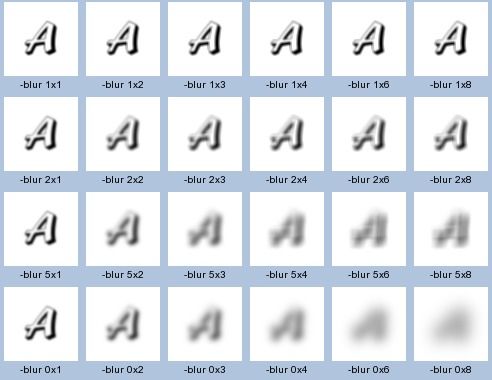
While the kernel can technically be an arbitrary size, we should scale σ in proportion to the kernel size. If we have a large kernel radius, but a small sigma, then all of the new pixels we’re introducing with our larger radius aren’t really affecting the computation. 

Here’s an example of a large kernel radius, but a small sigma: 

As opposed to Sigma 5, Kernel 111:

Code

To finish our implementation, we’ll also need to normalize the values in our kernel. Otherwise the image will become darker as the values will sum to slightly less than 1. Finally, we’ll need to make sure that the size of the kernel is odd to ensure that there is an actual center pixel. 

The code below is by no means the fastest and favors clarity over brevity:

Here’s the full implementation in Swift:

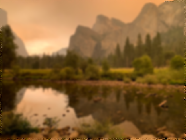
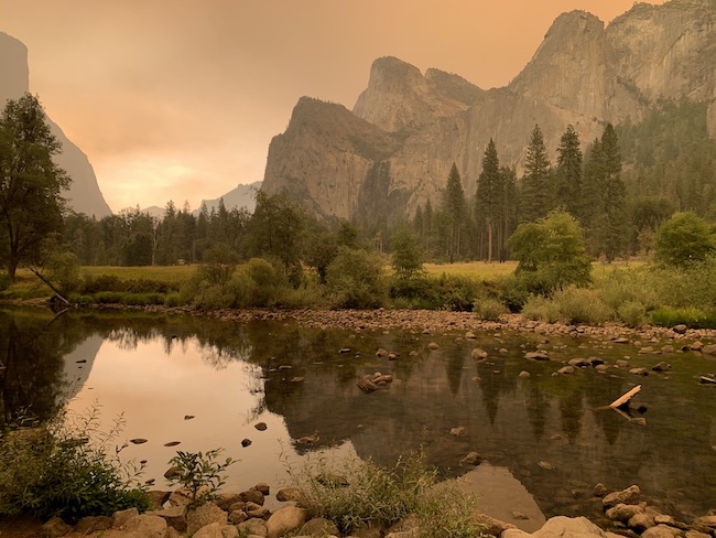
Here are some of the results on a photo I captured amidst Yosemite’s fires last weekend:

Original:

Radius: 3

Radius: 5

Radius: 11